Usage Examples

• Usage Examples
• • Quickstart
  • Quickly access and compare tables
  • Scaling and capping rates

Quickstart

Load and see information about a particular table:

julia> vbt2001 = MortalityTables.table("2001 VBT Residual Standard Select and Ultimate - Male Nonsmoker, ANB")
MortalityTable (Insured Lives Mortality):
   Name:
       2001 VBT Residual Standard Select and Ultimate - Male Nonsmoker, ANB
   Fields:
       (:select, :ultimate, :metadata)
   Provider:
       Society of Actuaries
   mort.SOA.org ID:
       1118
   mort.SOA.org link:
       https://mort.soa.org/ViewTable.aspx?&TableIdentity=1118
   Description:
       2001 Valuation Basic Table (VBT) Residual Standard Select and Ultimate Table -  Male Nonsmoker.
       Basis: Age Nearest Birthday. 
       Minimum Select Age: 0. 
       Maximum Select Age: 99. 
       Minimum Ultimate Age: 25. 
       Maximum Ultimate Age: 120

The package revolves around easy-to-access vectors which are indexed by attained age:

julia> vbt2001.select[35]          # vector of rates for issue age 35
 0.00036
 0.00048
 ⋮
 0.94729
 1.0
 
julia> vbt2001.select[35][35]      # issue age 35, attained age 35
 0.00036
 
julia> vbt2001.select[35][50:end] # issue age 35, attained age 50 through end of table
0.00316
0.00345
 ⋮
0.94729
1.0

julia> vbt2001.ultimate[95]        # ultimate vectors only need to be called with the attained age
 0.24298

Calculate the force of mortality or survival over a range of time:

julia> survival(vbt2001.ultimate,30,40) # the survival between ages 30 and 40
0.9894404665434904

julia> decrement(vbt2001.ultimate,30,40) # the decrement between ages 30 and 40
0.010559533456509618

Non-whole periods of time are supported when you specify the assumption (Constant(), Uniform(), or Balducci()) for fractional periods:

julia> survival(vbt2001.ultimate,30,40.5,Uniform()) # the survival between ages 30 and 40.5
0.9887676470262408

Quickly access and compare tables

This example shows how to develop a visual comparison of rates from scratch, but you may be interested in this pre-built tool for this purpose.

using MortalityTables, Plots


cso_2001 = MortalityTables.table("2001 CSO Super Preferred Select and Ultimate - Male Nonsmoker, ANB")
cso_2017 = MortalityTables.table("2017 Loaded CSO Preferred Structure Nonsmoker Super Preferred Male ANB")

issue_age = 80
mort = [
	cso_2001.select[issue_age][issue_age:end],
	cso_2017.select[issue_age][issue_age:end],
	     ]
plot(
	   mort,
	   label = ["2001 CSO" "2017 CSO"],
	   title = "Comparison of 2107 and 2001 CSO \n for SuperPref NS 80-year-old male",
	   xlabel="duration")

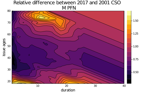
Easily extend the analysis to move up the ladder of abstraction:

issue_ages = 18:80
durations = 1:40

# compute the relative rates with the element-wise division ("broadcasting" in Julia)
function rel_diff(a, b, issue_age,duration)
        att_age = issue_age + duration - 1
        return a[issue_age][att_age] / b[issue_age][att_age]
end


diff = [rel_diff(cso_2017.select,cso_2001.select,ia,dur) for ia in issue_ages, dur in durations]
contour(durations,
        issue_ages,
        diff,
        xlabel="duration", ylabel="issue ages",
        title="Relative difference between 2017 and 2001 CSO \n M PFN",
        fill=true
        )

Scaling and capping rates

Say that you want to take a given mortality table, scale it by 130%, and cap it at 1.0. You can do this easily by broadcasting over the underlying rates (which is really just a vector of numbers at the end of the day):

issue_age = 30
m = cso_2001.select[issue_age]

scaled_m = min.(cso_2001.select[issue_age] .* 1.3, 1.0) # 130% and capped at 1.0 version of `m`

Note that min.(cso_2001.select .* 1.3, 1.0) won't work because cso_2001.select is still a vector-of-vectors (a vector for each issue age). You need to drill down to a given issue age or use an ultimate table to manipulate the rates in this way.